Assembly and Co-assembly of Metagenomic Raw Reads

Authors

Affiliation

Germana Baldi

EMBL-EBI

Tanya Gurbich

EMBL-EBI

Published

October 10, 2023

Learning Objectives

In the following exercises you will learn how to perform metagenomic assembly and co-assembly, and to start exploring the output. We will shortly observe assembly graphs with Bandage, peek into assembly statistics with assembly_stats, and align contig files against the BLAST database.

Note

The process of metagenomic assembly can take hours, if not days, to complete on a normal sample, as it often requires days of CPU time and 100s of GB of memory. In this practical, we will only be investigating very simple example datasets.

Once you have quality filtered your sequencing reads, you may want to perform de novo assembly in addition to, or as an alternative to read-based analyses. The first step is to assemble your sequences into contigs. There are many tools available for this, such as MetaVelvet, metaSPAdes, IDBA-UD, or MEGAHIT. We generally use metaSPAdes, as in most cases it yields the best contig size statistics (i.e. more continguous assembly), and it has been shown to be able to capture high degrees of community diversity (Vollmers, et al. PLOS One 2017). However, you should consider pros and cons of different assemblers, which not only includes the accuracy of the assembly, but also their computational overhead. Compare these factors to what you have available. For example, very diverse samples with a lot of sequence data (e.g. samples from the soil) uses a lot of memory with SPAdes. In the following practicals we will demonstrate the use of metaSPAdes on a small short-read sample, Flye on a long-read sample, and MEGAHIT to perform co-assembly.

Before we start…

Let’s first move to the root working directory to run all analyses:

cd /home/training/Assembly/

You will find all inputs needed for assemblies in the reads folder.

Note

If anything goes wrong during the practical, you will find assembly backups for all steps in the respective “.bak” folders.

Short-reads assemblies: metaSPAdes

For short reads, we will use SPAdes - St. Petersburg genome Assembler (https://github.com/ablab/spades), a suite of assembling tools containing different assembly pipelines. For metagenomic data, we will explore metaSPAdes. metaSPAdes offers many options that fit your preferences differently, mostly depending on the type of data you are willing to assemble. To explore them, type metaspades.py -h. Bear in mind that options will differ when selecting different tools (e.g. spades.py) and they should be tuned according to the input dataset and desired outcome.

Step

The default metaSPAdes pipeline executes an error correction step on the input fastqs. To run metaspades without the error correction step, execute the following commands:

mkdir assembly_spades
metaspades.py -t 4 --only-assembler -m 10 -1 reads/oral_human_example_1_splitaa_kneaddata_paired_1.fastq -2 reads/oral_human_example_1_splitaa_kneaddata_paired_2.fastq -o assembly_spades

Note

The execution will take up to 20 minutes. Grab a coffee or read through the materials!

Once the assembly has completed, you will see plenty of files, including intermediate ones, in the assembly_spades folder. contigs.fasta and scaffolds.fasta are the ones you are usually interested into for downstream analyses (e.g. binning and MAG generation). We will focus on contigs.fasta for this session, which is the same you are going to use in the coming practicals. Contigs in this file are ordered from the longest to the shortest. You can already try to infer a strong taxonomic signal at this stage with a quick blastn alignment.

Step

Take the first 100 lines of the sequence and perform a blast search at NCBI (https://blast.ncbi.nlm.nih.gov/Blast.cgi, choose Nucleotide:Nucleotide from the set of options). Leave all other options as default on the search page. To select the first 100 lines of the assembly perform the following:

head -n 101 assembly.bak/contigs.fasta

The resulting output is going to look like this: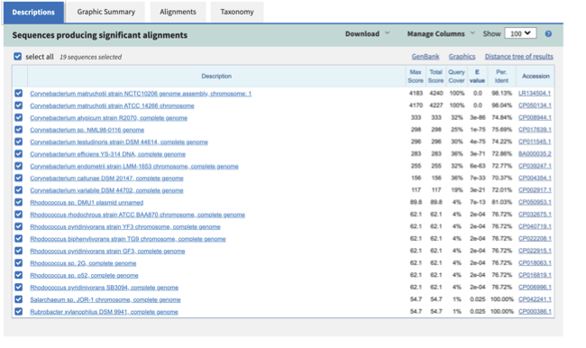

Question

Which species do you think this sequence may be coming from? Does this make sense as a human oral bacteria? Are you surprised by this result at all?

As mentioned in the theory talk, you might be interested in different statistics for your contigs file. assembly_stats is a tool that produces two simple tables in JSON format with various measures, including N10 to N50, GC content, longest contig length and more. The first section of the JSON corresponds to the scaffolds in the assembly, while the second corresponds to the contigs.

N50 is a measure to describe the quality of assembled genomes that are fragmented in contigs of different length. We can apply this with some caution to metagenomes, where we can use it to crudely assess the contig length covering 50% of the total assembly. Essentially, the longer the better, but this only makes sense when thinking about alike metagenomes. Note that N10 is the minimum contig length to cover 10 percent of the metagenome.

Step

assembly_stats assembly.bak/scaffolds.fasta

Question

What is the length of longest and shortest contigs?

What is the N50 of the assembly? Given that are input sequences were ~150bp long paired-end sequences, what does this tell you about the assembly?

Another tool to keep in mind for metagenomic assemblies is QUAST, which provides a deeper insight on assemblies statistics like indels and misassemblies rate in a very short time.

Long-reads assemblies: Flye

For long-reads, we will use Flye (https://github.com/fenderglass/Flye), which assembles single-molecule sequencing reads like PacBio and Oxford Nanopore Technologies (ONT) reads. As spades, Flye is a pipeline that takes care of assembly polishing. Similarly to assembly scaffolding, it tries to overcome long-reads base call error by comparing different reads that cover the same sequencing fragment. Flye’s parameters are quickly described in the help command (flye -h).

Flye supports metagenomic assemblies with the --meta flag. Backup assemblies for this section can be found in the Assembly folder, starting with “LR”.

Step

mkdir flye_out
flye --nano-raw reads/ONT_example.fastq --out-dir flye_out --threads 4

Extra

Note that we are not using the --meta flag. If you have some spare time, try to execute the same command with this flag and output folder “LR_meta_assembly”.

Note

Each execution will take around 5 minutes.

Let’s have a first look at how assembly graphs look like. Bandage (a Bioinformatics Application for Navigating De novo Assembly Graphs Easily) is a program that creates interactive visualisations of assembly graphs. They can be useful for finding sections of the graph, such as rRNA, or identify specific parts of a genome. Note, you can install Bandage on your local system. With Bandage, you can zoom and pan around the graph and search for sequences, and much more.

When looking at metaSPAdes output, it is usually recommended to launch Bandage on assembly_graph.fastg. However, our assembly is quite fragmented, so we will load assembly_graph_after_simplification.gfa.

We will use Bandage to compare the two assemblies we have generated, Flye and metaSPAdes.

Step

Bandage

In the Bandage GUI perform the following:

Select File -> Load graph
Navigate to Home/training/Data/Assembly/assembly.bak and open assembly_graph_after_simplification.gfa

Once loaded, you need to draw the graph. To do so, under the “Graph drawing” panel on the left side perform the following:

Set Scope to Entire graph
Click on Draw graph

Question

Can you find any large, complex parts of the metaSPAdes graph? If so, what do they look like?

Question

How does the Flye assembly differ from the one generated with metaSPAdes?

Extra

We launched Flye both with and without --meta on file reads/ONT_example.fastq. This file actually comes from run ERR3775163, which can be browsed on ENA (https://www.ebi.ac.uk/ena/browser/home). Have a look at sample metadata. Can you understand why, despite dealing with a long-read sample, the assembly graph looks better for the execution without the --meta option?

Extra

If you blast the first contig of the long-read assembly, do results match the metadata you find on ENA?

Co-assemblies: MEGAHIT

In the following steps of this exercise, we will perform co-assembly of multiple datasets. The first execution requires around 6-7 minutes to finish, the general suggestion is to run the first intruction and then rely on files in the coassembly.bak directory, which contains all expected results.

Step

First, make sure that output directories do not already exist, as MEGAHIT can’t overwrite existing directories. Bear in mind that backup assemblies for this exercise are in:

ls /home/training/Assembly/coassembly.bak

You can perform co-assemblies with MEGAHIT as follows:

megahit -1 reads/oral_human_example_1_splitaa_kneaddata_paired_1.fastq -2 reads/oral_human_example_1_splitaa_kneaddata_paired_2.fastq -o coassembly1_new -t 4 --k-list 23,51,77 

megahit -1 reads/oral_human_example_1_splitaa_kneaddata_paired_1.fastq,reads/oral_human_example_1_splitab_kneaddata_paired_1.fastq -2 reads/oral_human_example_1_splitaa_kneaddata_paired_2.fastq,reads/oral_human_example_1_splitab_kneaddata_paired_2.fastq -o coassembly2_new -t 4 --k-list 23,51,77 

megahit -1 reads/oral_human_example_1_splitaa_kneaddata_paired_1.fastq,reads/oral_human_example_1_splitab_kneaddata_paired_1.fastq,reads/oral_human_example_1_splitac_kneaddata_paired_1.fastq -2 reads/oral_human_example_1_splitaa_kneaddata_paired_2.fastq,reads/oral_human_example_1_splitab_kneaddata_paired_2.fastq,reads/oral_human_example_1_splitac_kneaddata_paired_2.fastq -o coassembly3_new -t 4 --k-list 23,51,77

You should now have three different co-assemblies generated from different subsamples of the same data.

Step

Compare the results of the three contig files with assembly_stats. How do these assemblies differ from the one generated previously with metaSPAdes? Which one do you think is best?

To generate assembly graphs for MEGAHIT output, execute:

megahit_toolkit contig2fastg 77 final.contigs.fa > final.contigs.fastg

… And now?

If you have reached the end of the practical and have some spare time, look at the paragraphs labelled “Extra”. They contain optional exercises for the curious student :)

…….. Yes, but now that I am really, really done?

You could try to assemble raw reads with different assemblers or parameters, and compare statistics and assembly graphs. Note, for example, that metaSPAdes can deal ONT data (but it will likely yield a lower quality assembly).

Reuse

Apache 2.0