Viral detection and classification
Varsha Kale 
Prerequisites
These instructions are for the course VM. To run externally please see the section at the end.
All commands detailed below will be run from within this current working directory. Note: if there are any issues in running this tutorial, there is a separate directory exp_results/ with pre-computed results.
1. Identification of putative viral sequences
In order to retrieve putative viral sequences from a set of metagenomic contigs, we are going to use two different tools designed for this purpose, each of which employs a different strategy for viral sequence detection: VirFinder and VirSorter. VirFinder uses a prediction model based on kmer profiles trained using a reference database of viral and prokaryotic sequences. In contrast, VirSorter mainly relies on the comparison of predicted proteins with a comprehensive database of viral proteins and profile HMMs. The VIRify pipeline uses both tools as they provide complementary results:
VirFinder performs better than VirSorter for short contigs (<3kb) and includes a prediction model suitable for detecting both eukaryotic and prokaryotic viruses (phages). In addition to reporting the presence of phage contigs, VirSorter detects and reports the presence of prophage sequences (phages integrated in contigs containing their prokaryotic hosts).
Lets look at the outputs of VirFinder. Look at the plot in the image below.
As you can see there is a relationship between the p-value and the score. A higher score or lower p-value indicates a higher likelihood of the sequence being a viral sequence. You will also notice that the results correlate with the contig length. The curves are slightly different depending on whether the contigs are > or < than 3kb. This is because VirFinder uses different machine learning models at these different levels of length.
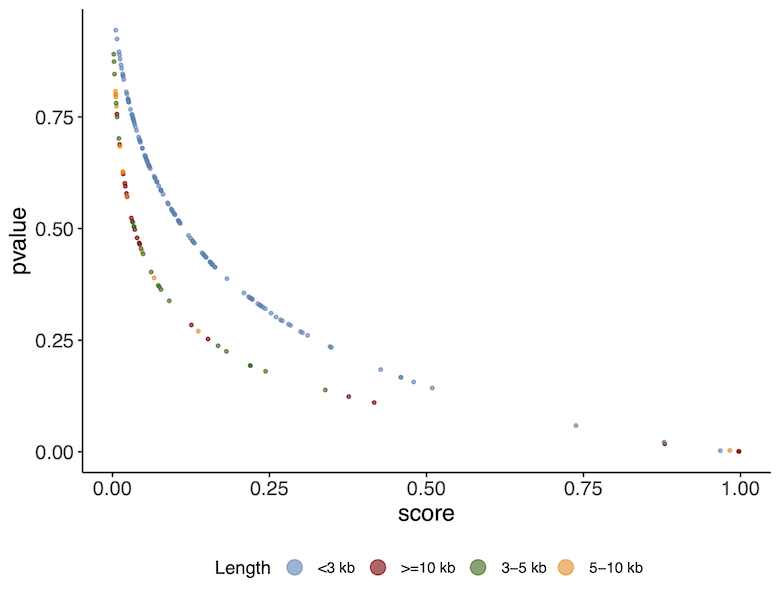
You will see a tabular file obs_results/ERR575691_virfinder.txt that collates the results obtained for each contig from the processed FASTA file.
If you wish to run this anytime after the practical, you will need to download the VirSorter database into the data/databases folder and then the following command can be used:
#DON'T RUN NOW
wrapper_phage_contigs_sorter_iPlant.pl -f obs_results/ERR575691_host_filtered_filt500bp_renamed_filt1500bp.fasta --db 2 --wdir obs_results/virsorter_output --virome --data-dir /opt/data/databases/virsorter-data
VirSorter classifies its predictions into different confidence categories:
- Category 1: “most confident” predictions
- Category 2: “likely” predictions
- Category 3: “possible” predictions
- Categories 4-6: predicted prophages
Following the execution of this command, FASTA files (*.fna) will be generated for each one of the VIRify categories mentioned above containing the corresponding putative viral sequences.
The VIRify pipeline takes the output from VirFinder and VirSorter, reporting three prediction categories:
- High confidence: VirSorter phage predictions from categories 1 and 2.
- Low confidence:
- Contigs that VirFinder reported with p-value < 0.05 and score ≥ 0.9.
- Contigs that VirFinder reported with p-value < 0.05 and score ≥ 0.7, but that are also reported by VirSorter in category 3.
- Prophages: VirSorter prophage predictions categories 4 and 5.
3. Viral taxonomic assignment
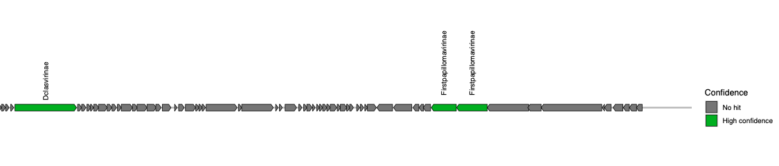
The final output of the VIRify pipeline includes a series of gene maps generated for each putative viral sequence and a tabular file that reports the taxonomic lineage assigned to each viral contig. The gene maps provide a convenient way of visualizing the taxonomic annotations obtained for each putative viral contig and compare the annotation results with the corresponding assigned taxonomic lineage. Taxonomic lineage assignment is carried out from the highest taxonomic rank (genus) to the lowest (order), taking all the corresponding annotations and assessing whether the most commonly reported one passes a pre-defined assignment threshold.
Final output results are stored in the obs_results/ directory.
The gene maps are stored per contig in individual PDF files (suffix names of the contigs indicate their level of confidence and category class obtained from VirSorter). Each protein coding sequence in the contig maps (PDFs) is coloured and labeled as high confidence (E-value < 0.1), low confidence (E-value > 0.1) or no hit, based on the matches to the HMM profiles. Do not confuse this with the high confidence or low confidence prediction of VIRify for the whole contig.
Taxonomic annotation results per classification category are stored as text in the *taxonomy.tsv files.
You should see a list of 9 contigs detected as viral and their taxonomic annotation in separate columns (partitioned by taxonomic rank). However, some do not have an annotation (e.g. NODE_4… and NODE_5…).
Now on your computer on the left hand bar, select the folder icon.
Navigate to Home –> virify_tutorial –> obs_results
Open the gene map PDF files of the corresponding contigs to understand why some contigs were not assigned to a taxonomic lineage. You will see that for these cases, either there were not enough genes matching the HMMs, or there was disagreement in their assignment.
Running the practical externally
We need to set up our computing environment in order to execute the commands above. Download the virify_tutorial_2023.tar.gz file containing all the data you will need using any of the following options:
    wget http://ftp.ebi.ac.uk/pub/databases/metagenomics/mgnify_courses/ebi_2023/virify_tutorial_2023.tar.gz
    #or
    rsync -av --partial --progress rsync://ftp.ebi.ac.uk/pub/databases/metagenomics/mgnify_courses/ebi_2023/virify_tutorial_2023.tar.gz .
Once downloaded, extract the files from the tarball:
tar -xzvf virify_tutorial_2023.tar.gzNow change into the virify_tutorial directory and setup the docker container by running the following commands in your terminal session:
    cd virify_tutorial
    docker pull quay.io/microbiome-informatics/2023-metagenomics-course-virify:1.0
    docker run --rm -it -v $(pwd):/opt/data quay.io/microbiome-informatics/2023-metagenomics-course-virify:1.0
    mkdir obs_results
The container has the following tools installed: - Python - R - VirSorter - VirFinder
All scripts and databases used can be found in the data folder.
You can now start from section 1 above.